The Design & Implementation of the CPython Virtual Machine
A deep dive into CPython's bytecode instruction format and execution engine internals
For every bytecode compiled language, the most interesting part of its implementation is its virtual machine (also referred to as the bytecode interpreter) where the bytecode execution takes place. Because this is such a crucial part of the language machinery, its implementation has to be highly performant. Even if you are not a compiler engineer, learning about such internal implementation can give you new performance tricks and insights that you may be able to use in other places of your job. And, if you are a compiler engineer then you should always look around how other languages are implemented to pickup implementation details that you may not be aware of.
In this article, we are going to be discussing the bytecode instruction format of CPython, followed by the implementation of the bytecode dispatch loop of the interpreter where the bytecode execution takes place.
The Design of Bytecode Virtual Machines
When it comes to compiled programming languages, the compiler’s job is to translate the code from the source language to the instructions of a target machine. This target machine can be a real hardware, such as X86, arm, riscv which come with a predefined set of instructions that they can execute.
Generating code for these different hardware architectures is complicated. But more importantly, it also poses portability issues—the code compiled for a particular processor architecture will only run on those kinds of machines, and to run the same program on a different architecture, the code needs to be recompiled.
As a result of these complications, many programming languages started to use virtual machines (VM). A virtual machine is an emulated machine implemented in software and it supports instructions similar to an actual hardware machine. The compiler’s job is to translate the source code to these instructions. Compiling programs for such a virtual machine is much simpler and it also solves the portability problems (the program once compiled can be run on any hardware where there is a virtual machine implementation available).
Python also comes with a similar virtual machine and Python’s compiler generates instructions (also called bytecode) for it.
Types of Virtual Machines
Similar to real hardware machines, there are two kinds of virtual machine implementations. We can have register based virtual machines where the instructions use registers for storing the operands for the instructions. Most modern hardware machines these days are also register based. These machines usually offer better performance, but are challenging to implement from the compiler’s point of view because of problems like register allocation.
The alternative to this design is a stack based VM. The instructions push and pop operands from the stack to perform their operations. This is a much simpler scheme, and the instructions are also very simple for the compiler to generate.
In the case of Python, it implements a stack based virtual machine. Other notable languages which use stack are Ruby, JavaScript, Java.
Bytecode Instructions
Now, let’s talk about how the instructions for these virtual machines look like and how they are packed in the form of bytecode. We will look at a hypothetical stack based VM which supports the following six instructions:
PUSH <value> # pushes the given value onto the stack
ADD # pops top two values from the stack, adds them and pushes result back onto the stack
SUB
MUL
DIV
HALT # Marks the end of the program and current stack top becomes return value
Each of these instructions can be assigned an integer opcode. For instance:
PUSH: 0
ADD: 1
SUB: 2
MUL: 3
DIV: 4
HALT: 5
As the compiler generates code for this VM, it will emit one of these opcode values depending on the type of operation being performed. For instance, if it is compiling an expression such as “1 + 2”, it will want to generate the following sequence of opcodes:
PUSH 1
PUSH 2
ADD
HALT
The two PUSH instructions will push the operands onto the stack and the ADD instruction will pop them from the stack, add them together and push the result onto the stack.
However, instead of generating the instructions in text format like above, the compiler would generate the actual opcodes for each instruction. So it would actually look like this:
0|0|1|60 is the opcode for PUSH, 1 is the opcode for ADD and 6 is for HALT.
As this VM only supports six instructions, 1 byte is sufficient to encode each of these instructions. But the PUSH instruction needs an argument which needs to be accommodated in the bytecode.
We can support an argument for the PUSH instruction by increasing its width to 2 bytes—the first byte represents the opcode and the 2nd byte is its argument value (a 1 byte argument means we can only push values up to 255 on the stack but that’s ok for a hypothetical toy VM).
This variable width instruction scheme would work but it would make the implementation of the VM a bit complicated. We can further simplify things by requiring all instructions to be 2 bytes wide where the first byte is the opcode and the 2nd is the optional argument which can be 0 if there is no argument value. Based on this specification the bytecode for the above program would become this:
0 1|0 2|1 0|6 0(I’ve used the |character to highlight the individual instruction boundaries).
The above sequence of bytes is called the bytecode and the virtual machine’s task is to unpack the instructions from this sequence of bytes and execute them.
Execution of the Bytecode in a Virtual Machine
Now, let’s talk about how the virtual machine unpacks and executes this bytecode. We will continue the example of our simple stack based VM from the previous section which supports only six instructions.
The following code shows how such a VM might evaluate the bytecode.
class VirtualMachine():
    def __init__(self, bytecode):
        self.stack = []
        self.bytecode = bytecode

    def execute_bytecode(self):
        ip = 0
        while ip < len(self.bytecode) - 1:
            opcode = self.bytecode[ip]
            oparg = self.bytecode[ip + 1]
            ip += 2
            match opcode:
                case PUSH:
                    self.stack.append(oparg)
                case ADD:
                    lhs = self.stack.pop()
                    rhs = self.stack.pop()
                    result = lhs + rhs
                    self.stack.append(result)
                case SUB:
                    lhs = self.stack.pop()
                    rhs = self.stack.pop()
                    result = lhs - rhs
                    self.stack.append(result)
                case MUL:
                    lhs = self.stack.pop()
                    rhs = self.stack.pop()
                    result = lhs * rhs
                    self.stack.append(result)
                case DIV:
                    lhs = self.stack.pop()
                    rhs = self.stack.pop()
                    result = lhs / rhs
                    self.stack.append(result)
                case HALT:
                    return stack.pop()
The VM runs a loop through the bytecode instructions and based on the value of the opcode, performs the right operation.
This is a deliberately simple code to illustrate the main principles of fetching, decoding and executing instructions. For instance, this VM is capable of only working with integer values which are received as arguments to the instructions and directly pushed to the stack. A real-world VM implementation has a ton of more details such as stack frames, stack pointer, instruction pointer, execution context, which I have excluded here. We will discuss these as we get into the CPython VM implementation details.
The Implementation of the CPython Virtual Machine
At this point we understand how a bytecode virtual machine works (in principle). Now, we are ready to discuss the specifics of CPython’s VM implementation.
CPython Bytecode Instructions
We will start by looking at the instructions that the Python virtual machine supports and then discuss how they are packed in the form of bytecode.
In CPython, the instruction opcodes are defined in the file Include/opcode_ids.h. The following picture shows some of these instructions and their associated opcode ids.
At the time of writing this article (CPython 3.14 in development), CPython has a total of 223 instructions defined.
Note: This file is generated via a script, the actual instructions are defined in the file Python/bytecodes.c. In fact, most of the VM implementation is generated using different scripts by parsing the instruction definitions in this file.
CPython Bytecode Packing Format
Similar to the toy example we discussed from the previous section, the CPython bytecode instructions are also two bytes wide. The first byte represents the opcode, and the 2nd byte represents argument value for that opcode. If the instruction does not expect any argument, the 2nd byte is set to 0.
However, having only a 1 byte wide argument means that the value cannot be larger than 255. To support larger argument values, there is a special instruction called EXTENDED_ARG. If the compiler notices that the argument value of an instruction cannot fit into a single unsigned byte, it emits the EXTENDED_ARG instruction for the extra set of bytes required to hold the argument value.
An instruction can be prefixed by a maximum of three consecutive EXTENDED_ARG instructions. This implies that the maximum argument size for an instruction is limited to 4 bytes (1 byte argument to the instruction itself, and 3 bytes via the three EXTENDED_ARG instructions).
Understanding the CPython Bytecode With an Example
Let’s consider an example function and see its generated bytecode to understand this better.
>>> def add(a, b):
...     return a + b
...
>>> dis.dis(add)
  1           RESUME                   0

  2           LOAD_FAST_LOAD_FAST      1 (a, b)
              BINARY_OP                0 (+)
              RETURN_VALUE
We have a simple function to add two values, and we can see its generated bytecode instructions using the dis module.
We can also inspect the actual bytecode of this function. Every callable object in Python has a __code__ field which contains a field _co_code_adaptive that contains the compiled bytecode for that object. Let’s inspect it.
>>> add_bytecode = add.__code__._co_code_adaptive
>>> len(add_bytecode)
10
>>> for i in range(0, len(add_bytecode) - 1, 2):
        print(f"opcode_value: {add_bytecode[i]}, oparg: add_bytecode[i+1]}")

opcode_value: 149, oparg: 0
opcode_value: 88, oparg: 1
opcode_value: 45, oparg: 0
opcode_value: 0, oparg: 0
opcode_value: 36, oparg: 0
>>>
We see that the bytecode is indeed a sequence of bytes. And, we have printed the individual instructions and their arguments by iterating over each pair of the bytes in that sequence.
Notice that the output of
dis.dis()showed 4 instructions, which means the bytecode should be 8 bytes long. However, the generated bytecode is 10 bytes long. This is because there is an extraCACHEinstruction (opcode 0) generated by the compiler which is not shown in the default output of dis.dis(). TheCACHEinstruction is used as an inline data cache for optimizing certain instructions by the VM. CPython profiles and optimizes certain instructions to more specialized versions for improving performance. We will talk about how this instruction specialization works in a future article.
We can also go one step ahead and decode these opcode values to see that they match the instructions as printed by the dis module.
>>> import opcode
>>> for i in range(0, len(add_bytecode) - 1, 2):
...     opcode_value, oparg = add_bytecode[i], add_bytecode[i + 1]
...     print(f"opcode_value: {opcode_value}, opcode_name: {opcode.opname[opcode_value]}, oparg: {oparg}")
...
opcode_value: 149, opcode_name: RESUME, oparg: 0
opcode_value: 88, opcode_name: LOAD_FAST_LOAD_FAST, oparg: 1
opcode_value: 45, opcode_name: BINARY_OP, oparg: 0
opcode_value: 0, opcode_name: CACHE, oparg: 0
opcode_value: 36, opcode_name: RETURN_VALUE, oparg: 0
>>>To decode the instructions, we’ve used the opcode module which contains mapping of opcode ids and their names. We can see that the opcode values match with the instruction names. Alternatively, you can also open the opcode_ids.h file and check the opcode names for the ids in the above bytecode.
The CPython Virtual Machine Internals
Now, let’s start diving into the implementation of CPython’s virtual machine. When we execute a new Python program, a lot of things happens before the virtual machine starts to execute the bytecode, such as runtime initialization, parsing and compilation of the code, stack frame setup etc.
The bytecode dispatch loop is itself complicated enough that there is not enough space in this article to cover these things, as a result I had to move this part to another article. If you are interested in learning about these details, you should check out that article linked below:
In this article, we are going to directly jump to the bytecode dispatch loop which is implemented in the function _PyEval_EvalFrameDefault in the file ceval.c. The following figure shows its signature.

This function receives the stack frame of the Python code block which is going to be executed on the VM. A stack frame holds the compiled bytecode and the necessary context for the VM to execute that bytecode.
This function unpacks the bytecode from the stack frame and starts evaluating it using the dispatch loop. Before we look at the body of this function it is important that we understand stack frames well, and also understand the concept of computed goto which is used by CPython to implement the dispatch loop.
Understanding Stack Frames
A stack frame is a construct designed to isolate the execution of a code block. For instance, when executing a function, the local variables and parameters of that function should only be visible within the context of that function. The caller should not be able to see or modify this local context. Similarly, no other parallely executing thread executing the same function should have access to this local data of another thread. The stack frame provides this isolation.
So, how does this work? You encapsulate the execution context of a block of code within the stack frame object. In Python, the execution context includes data such as the local objects, global objects, builtins, and also the stack where the VM will store the data while executing instructions for that code block.
Apart from that, the stack frame also enables the implementation of the call stack. Whenever you call a function, you first create a new stack frame for the called function and you link the caller’s stack frame to the callee’s stack frame like a linked list. Whichever function is currently executing becomes the head of this linked list. At any point of time, you can traverse this linked list to generate the stack trace of the current thread. Tools such as debuggers and profilers depend on this.
Now let’s see how stack frames are implemented in CPython.
Stack Frame Implementation in CPython
In CPython, the stack frame is defined as a C struct whose definition is shown in the diagram below.
You can clearly see how it encapsulates all the relevant execution context. Let’s discuss what are some of the key fields.
f_executable
:This contains the compiled bytecode for the block.previous: This is a pointer to the caller’s stack frame. The stack frames of the caller and callee functions are linked using it which creates the call stack.
globals: This is a dictionary containing all the global objects in the context of the current stack frame. The runtime automatically populates this dictionary while creating the stack frame.
locals: This is the dictionary where the local variables and function call arguments are stored.
builtins: This is the dictionary containing all the builtins available for use in the current stack frame’s context.
instr_ptr: Every stack frame has an instruction pointer which points to the next instruction to be executed. This maintains the state of the thread. For instance, if the VM switches to another thread, then the VM will know where the execution was paused.
stacktop: This is the offset to the top of the stack.
localsplus: This is an interesting field. It is used as a storage for holding local objects, and also as the stack for this block. The first x ( where x is the number of locals in the block) entries of the array are reserved for use as the locals list and the space after that is used as the stack. The CPython compiler tries to optimize access to local objects by generating instructions, such as
LOAD_FASTthat accesses this list using integer indices, which is much faster than doing a hash-based lookup in the locals dictionary.
Stack Frames with an Example
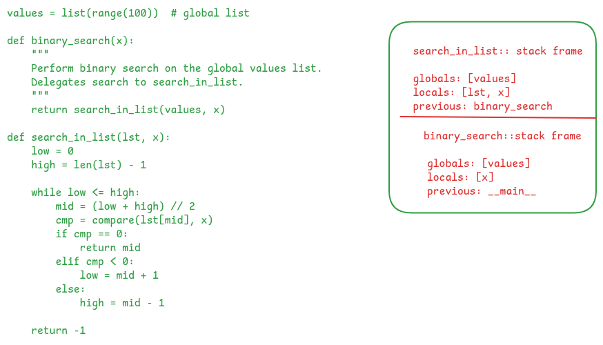
Let’s concretize our understanding of stack frames with an example. The following figure shows Python code which creates a global list object and a binary_search function to search through it. When this function is executed, a stack frame will be created for it which will contain the bytecode for the function body, and also the related data to execute that code.

We see that the binary_search function calls another function: search_in_list and passes it the values object and the x value as parameter. Again, when this function is called, a new stack frame will be created for it. This stack frame will contain the parameters as part of the locals dictionary. You will also notice that the previous field is linked to the caller’s stack frame.
Finally, the search_in_list function calls the cmp function in a loop. Every time cmp is called, a new stack frame is created for its execution in a similar manner. The following figure shows the call stack when it is called.
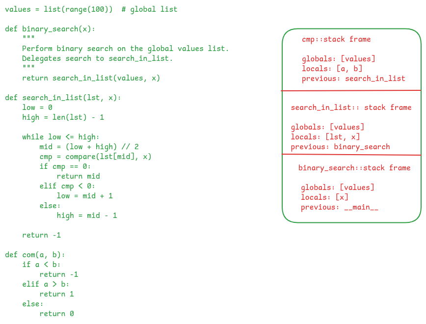
Hopefully, this example solidifies the role and importance of stack frames in the execution of code blocks in Python. It is central to how the CPython VM works. Now let’s discuss another important concept related to how the CPython VM implements the bytecode dispatch loop, which is computed gotos.
Switch Case vs Computed Goto based Dispatch Loop
Another thing we need to get acquainted with before we start to discuss the CPython VM code, is the concept of computed goto.
As we saw in the implementation of the toy VM, the dispatch loop is typically implemented using a switch case. In the case of CPython it looks something like the following:
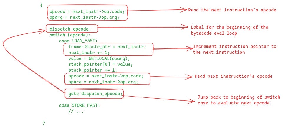
Note that the actual CPython bytecode eval loop is implemented using macros. The above picture is showing how the switch-based implementation looks like after macro expansion.
This is pretty straightforward to understand. There is no explicit while or for loop. Instead, a label dispatch_opcode is defined at the beginning of the switch block. Every opcode jumps back to this label after finishing its execution to execute the next opcode, which forms a loop.
In the above figure, I’ve shown the code for the LOAD_FAST instruction to illustrate the loop in action. The LOAD_FAST instruction is used to load a value from the locals list onto the stack. After doing this, it increments the instruction pointer to read the next opcode value and then jumps to the beginning of switch case to evaluate the new opcode.
Performance Limitations of Switch-based Dispatch Loop
Although the switch-based dispatch loop implementation is simple, it is problematic from a performance point of view.
At the beginning of every iteration of the loop, the decision of selecting the next case block depends on the value of the opcode. The CPU typically executes multiple instructions in parallel for better hardware utilization. To do this, it needs to find independent instructions that can be executed in parallel, and for this the CPU scans a window of program instructions.
The switch-based code requires comparing the opcode value and then jump to the code where the opcode’s implementation is present. Instead of waiting for the result of the comparison to be known, the CPU uses branch predictor to predict the likely target of the jump and starts executing instructions at that address.
Branch predictors are hardware units which learn the branching pattern from historical execution of a jump instruction. In the case of a switch-based implementation, there is a single jump instruction whose target constantly changes with the opcode value and it becomes harder for the branch predictor to predict the jump targets for it. Branch predictors do well, when the branching patterns are more predictable.
Computed goto based Dispatch Loop
A branch predictor friendly implementation of the dispatch loop is possible via the computed goto construct. Computed goto is a C compiler extension supported by a few compilers, such as clang and GCC. It allows us to use the special && operator to get the addresses of the labels in the C code.
The CPython VM implementation code assigns a unique label to the implementation of each opcode and then generates a static jump table using the addresses of these labels. At bytecode evaluation time, the VM does a lookup of this table using the opcode id and jumps to that address.
The following figure shows how the CPython VM uses computed gotos for implementing the dispatch loop:
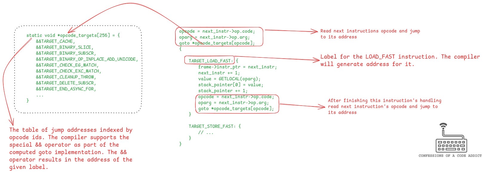
&& operator to get these addresses. The evaluation loop simply looks up this table using the opcode id and jumps to it to execute the code for that opcode.This implementation offers much improved performance over the switch case based implementation because the branch predictor can do a much better job with this scheme. Exactly why it offers better performance requires understanding how the branch predictor works, we will dive into it in another post (or maybe join my next live session to understand it).
CPython’s Bytecode Dispatch Loop
Because of its superior performance, computed goto is the preferred way to implement the bytecode dispatch loop, but not all the compilers support it. As a result the CPython implementation of the loop is done using preprocessor macros which can generate the code for switch case, or computed goto, depending on whether the compiler supports computed goto or not.
The following figure shows the code from the _PyEval_EvalFrameDefault function and effectively this results in the bytecode dispatch loop. It doesn’t look like a loop because of the macro magic but we will decode it now.
To understand this code we will break it down into two parts. The first part will explain the code before the loop (the prelude) and then 2nd part will explain the macros which generate the loop.
Prelude to the loop
In the above figure, all the code until the DISPATCH() call forms the prelude to the dispatch loop where some key variables and objects are initialized to track the state of the VM as it executes the bytecode.
Let’s break it down:
The
opcodeandopargvariables hold the next bytecode instruction and its argument values. These will continue to get updated at each iteration of the loop.Next, the
entry_frameobject is initialized and set as the previous frame to the frame which is going to be executed. This makesentry_framethe bottommost frame on the interpreter. It is executed at the end when all the Python code has finished executing. It contains bytecode instructions that tell the VM to exit the dispatch loop. We will see how this plays out after we finish discussing the dispatch loop.next_instris the instruction pointer which always points to the next instruction which is to be executed. It is initialized to the current frame’s instruction pointer value. When the VM changes the currently active frame (e.g. when calling a function), this variable is also updated to use the new frame’s instruction pointer value.
After this the body of the dispatch loop starts which heavily depends on the use of macros. Let’s understand it in detail.
The Loop Macros
The bytecode dispatch loop is implemented exactly the same way as what we saw in the section on computed goto vs switch case, but it is written using macros so that if the compiler doesn’t support computed gotos then the macros expand into switch cases, otherwise they expand into the computed goto based code. To understand the loop implementation we need to talk about the macro definitions that it uses.
The figure down below shows the definitions of the macros. These macros collectively expand into the code for one iteration of the loop. At every iteration of the loop the following things need to happen:
We need to get the opcode of the next instruction which is achieved using the
NEXTOPARG()macro.After that, we need to jump to the opcode implementation to execute it. This is achieved using the
DISPATCH_GOTO()macro. If computed goto is not being used then it expands into a jump to the beginning of the switch block. However, if computed goto is being used then it expands into a lookup of theopcode_targetsjump table and jump to the opcode implementation.
Both of these steps are combined into a single macro called DISPATCH(). So, whenever you see a DISPATCH() call in the code, it means that the next opcode is being fetched and executed.

Also, notice the TARGET(op) macro here. It takes the opcode as an argument and expands into either “TARGET_op:”, or “case op: TARGET_op”, depending on whether computed gotos are being used or not. It is used to start the body of each opcode’s implementation.
The Loop Body
Now we are ready to discuss the loop body. The following figure shows the code.
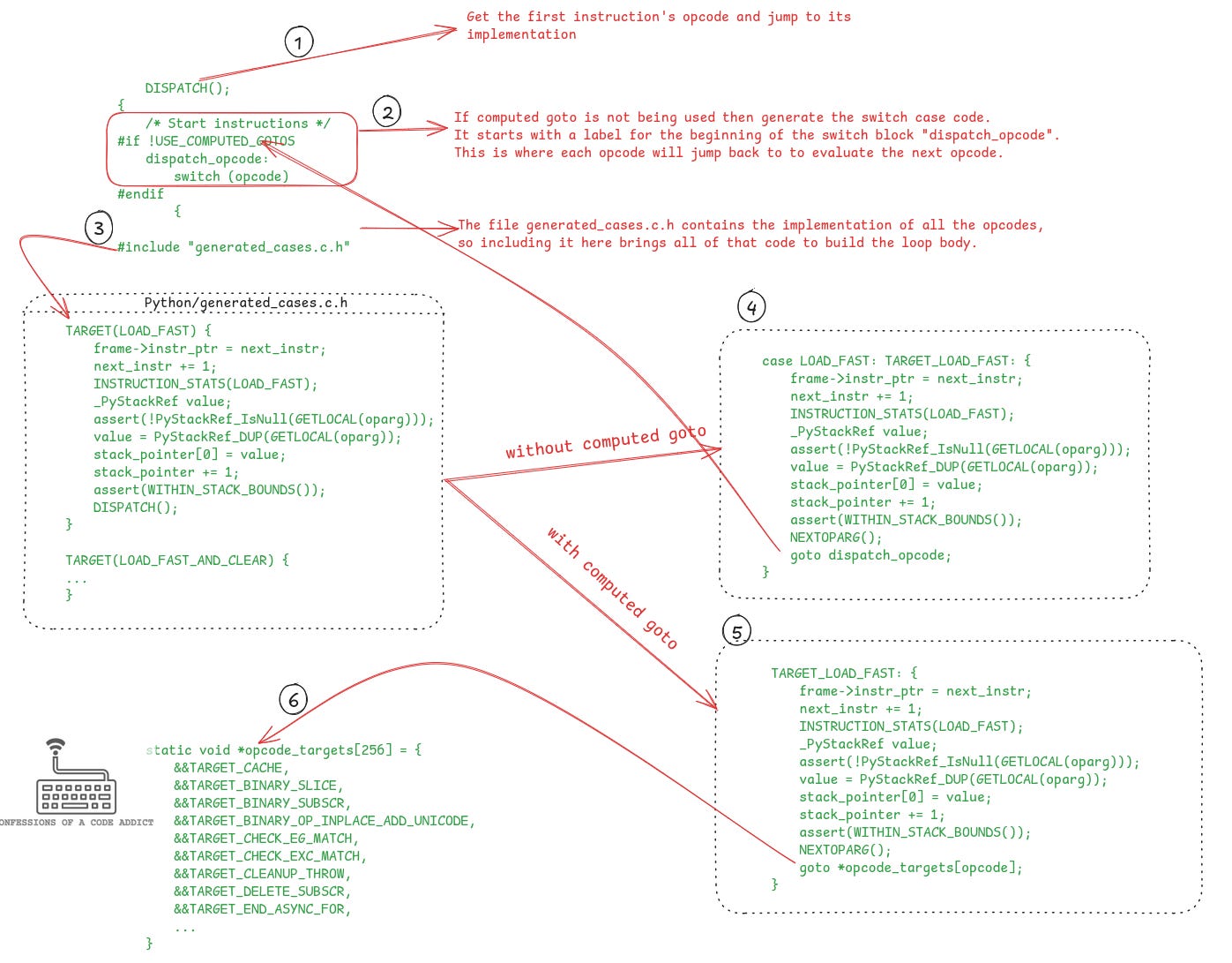
Let’s understand what is happening here. I will explain each of the numbered parts of the figure one by one.
The
DISPATCH()call gets the first opcode and jumps to its implementation. If using computed goto, the jump is to the label where the opcode is implemented using the jump table; otherwise it uses the switch case.If computed goto is not being used then the conditional compilation code generates the beginning of the switch block and also assigns it the label “
dispatch_opcode”.Next, it includes the file generated_cases.c.h where all the opcodes are implemented. The figure shows the implementation of the
LOAD_FASTinstruction from that file as an example. You can see it starts with theTARGETmacro that we discussed previously.If computed goto is not being used then the
TARGET(LOAD_FAST)macro call expands into “case LOAD_FAST: TARGET_LOAD_FAST:”. This forms the beginning of the case block. I’ve shown how the generated switch case looks like on the right hand side. Notice that at the end of the case block, there is a jump to the beginning of the switch block using thegotostatement. This forms a loop which continues as long as there are instructions to execute.If computed goto is being used then
TARGET(LOAD_FAST)expands into the labelTARGET_LOAD_FASTand the implementation of opcode will be under that label. I’ve shown the generated code on the right hand side. Again, notice that at the end of the code it fetches the opcode for the next instruction and then jumps to its implementation using the jump table. This is how a loop is formed in the case of computed goto based implementation.
The following figure shows the generated code for the switch case based loop and the computed goto based loop side by side.

Execution of a Python Program on the CPython VM
So far we have seen the implementation of the bytecode dispatch loop in the CPython VM. Let’s round things up by going through a sample Python program and understand how it would execute on the VM. This should solidify all the things we have talked about in the article.
We will use the following code as an example to step through the VM.
>>> def add(a, b):
    return a + b

>>> add(2, 3)
>>> dis.dis("add(2,3)")
  0           RESUME                   0

  1           LOAD_NAME                0 (add)
              PUSH_NULL
              LOAD_CONST               0 (2)
              LOAD_CONST               1 (3)
              CALL                     2
              RETURN_VALUE
The program is a single line of Python code calling the add function with the arguments 2 and 3. We can also see the compiled bytecode instructions for this one line program that will execute on the VM.
To execute this compiled code on the interpreter, it will be wrapped in a stack frame and passed to the _PyEval_EvalFrameDefault function for evaluation.
Recall that in _PyEval_EvalFrameDefault, before the dispatch loop starts, an entry_frame object is created which becomes the bottommost stack frame on the interpreter. The following figure shows how this looks like visually:
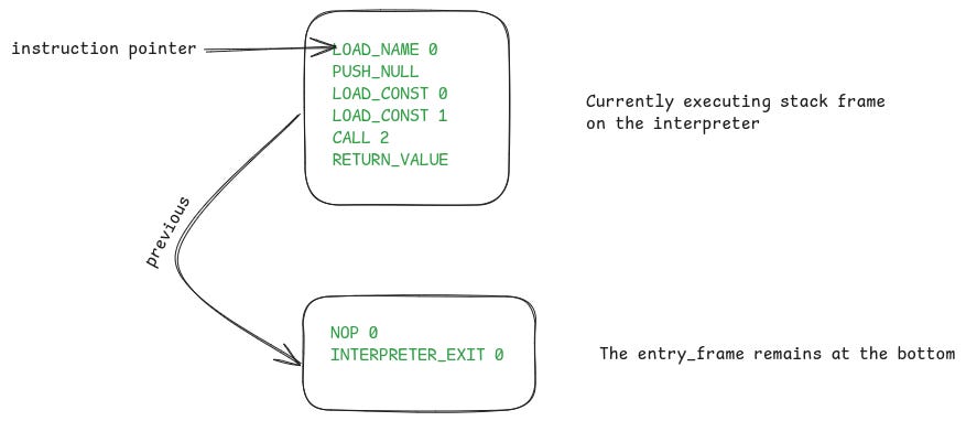
Initially, the VM’s instruction pointer will point to the first instruction LOAD_NAME. Next, the interpreter will enter the dispatch loop and evaluate each instruction one by one. The CALL instruction is where things get interesting.
The CALL instruction performs a function call. To do that it creates a new stack frame for the called function (the callee) and makes it the active stack frame. It also updates the instruction pointer variable to point to the callee’s first instruction, and finally jumps back to the beginning of the dispatch loop to start executing the callee’s code. Following diagram shows how the things will look like after the CALL instruction finishes.
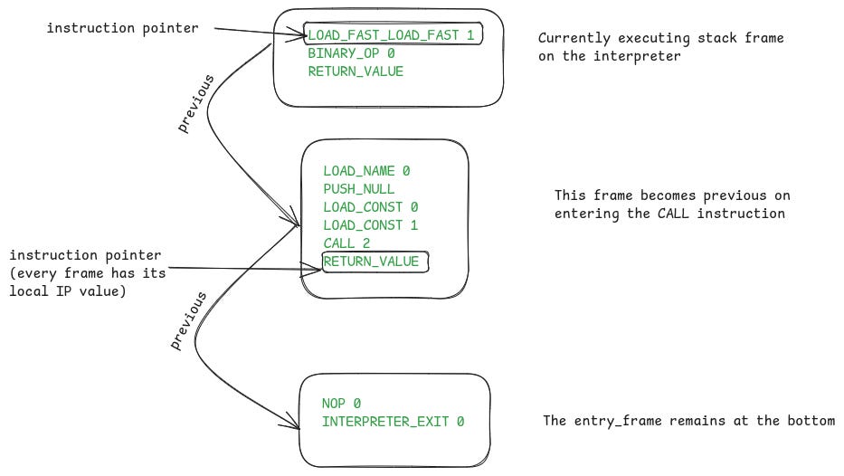
Note that, every function’s stack frame has its own private instruction pointer and stack pointer values. At this point the caller frame’s instruction pointer points to the
RETURN_VALUEinstruction where the VM will return to after theaddfunction finishes execution.
Again, the instructions of the add function will be evaluated one by one. When the execution reaches the RETURN_VALUE instruction then its stack frame will get popped and control will return to the caller. The following figure shows the code of the RETURN_VALUE instruction
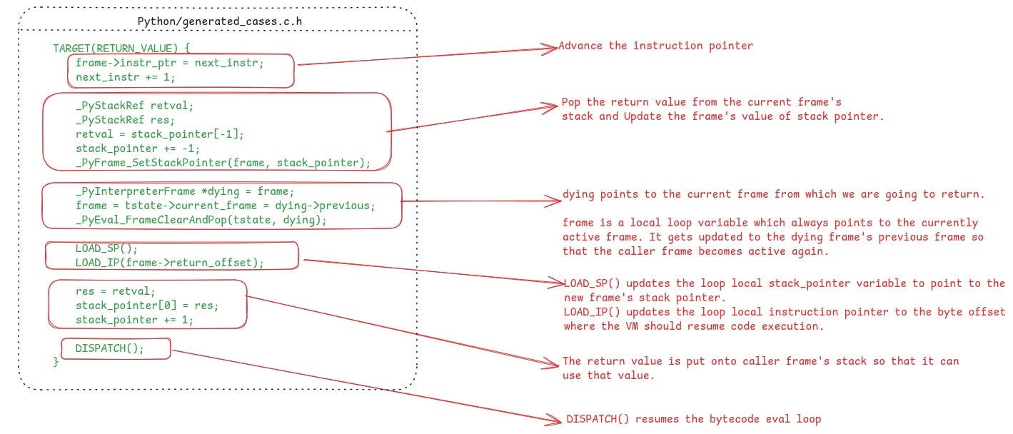
RETURN_VALUE instruction which pops the callee function’s stack frame and returns control back to the caller.
As you can see it takes the return value from the callee’s stack, then pops the stack frame so that the caller’s stack frame becomes active again, and finally updates the VM’s stack pointer and instruction pointers to point to the caller frame’s stack pointer and instruction pointer values respectively.
The following figure shows the status of the stack frames on the interpreter after the RETURN_VALUE instruction finishes.
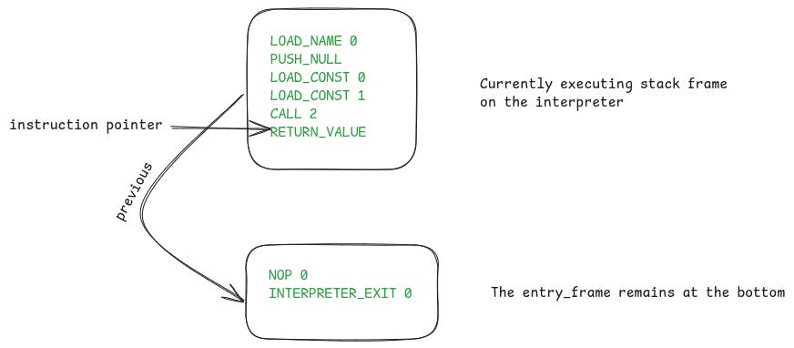
The control will return to the previous frame to execute its next instruction, which in this case is the RETURN_VALUE instruction. Again, similar set of things will happen. This frame will be popped and the entry_frame will become the active frame.

The entry_frame has only two instructions to execute. The NOP instruction doesn’t do anything so the instruction pointer will move on to the INTERPRETER_EXIT instruction which will end the dispatch loop and exit the interpreter. The following listing shows its implementation.
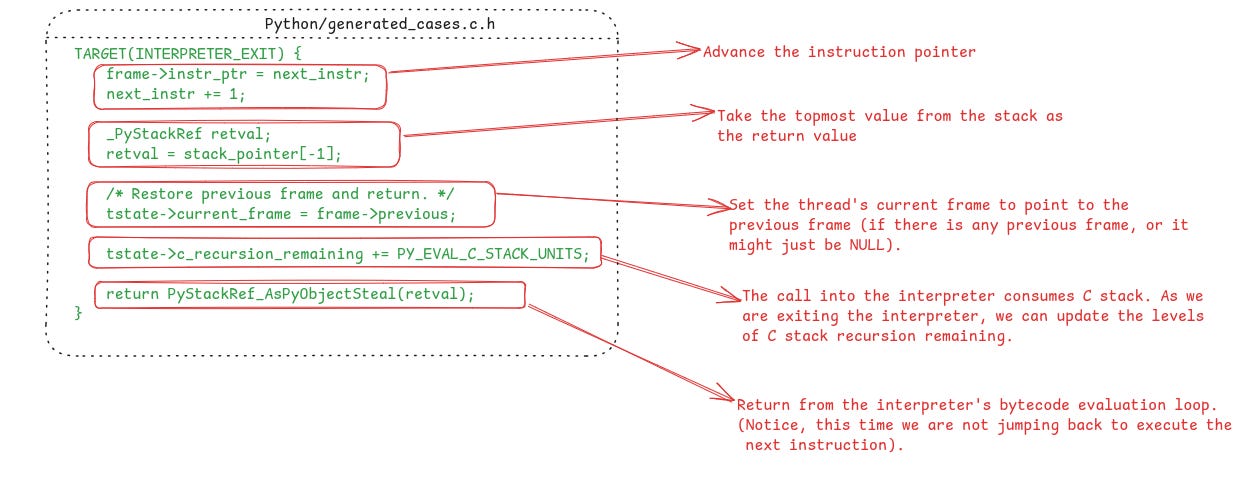
Notice unlike the other instructions which end with a goto statement to continue the loop, INTERPRETER_EXIT ends with a return statement. This makes the VM terminate the dispatch loop and return from the _PyEval_EvalFrameDefault. This ends the Python program execution as well, the return value of the executed code block is returned to from where the VM was invoked.
Summary
This brings us to a logical conclusion of this article. We started from a broad discussion of bytecode virtual machines, looked at the nitty gritty implementation details of bytecode execution in CPython and ended up with a walkthrough of a tiny Python program to see how all of this ties up. The following is a quick summary of everything we discussed in this article.
Bytecode and Virtual Machines: We started off by discussing how compiled languages use virtual machines to execute bytecode, making code portable across different hardware.
Types of VMs: We looked at two types of virtual machines – register-based and stack-based. Python uses a stack-based VM, just like Java and JavaScript.
Bytecode Format: We explored how bytecode instructions are packed, specifically for a hypothetical stack-based VM with a few basic instructions.
Execution Loop: We walked through how a virtual machine (like our example VM) processes and executes these bytecode instructions.
CPython Specifics: We jumped into the actual CPython VM, discussing its bytecode instructions and how they're organized.
Stack Frames: We broke down stack frames and their role in the VM, showing how each function call gets its own frame, helping the VM keep track of where it is.
Computed Goto: We explained why CPython uses computed gotos for better performance over traditional switch-case statements in the bytecode dispatch loop.
Putting It All Together: We took a sample Python program and walked through how the CPython VM executes it, detailing what happens step-by-step.
Support Confessions of a Code Addict
If you find my work interesting and valuable, you can support me by opting for a paid subscription (it’s $6 monthly/$60 annual). As a bonus you get access to monthly live sessions, and all the past recordings.
Many people report failed payments, or don’t want a recurring subscription. For that I also have a buymeacoffee page. Where you can buy me coffees or become a member. I will upgrade you to a paid subscription for the equivalent duration here.
I also have a GitHub Sponsor page. You will get a sponsorship badge, and also a complementary paid subscription here.
Free PDF Download for Subscribers
Paid subscribers can use the code below to download a complimentary PDF version of the article.


