Looking Under the Hood of Python's Set Data Structure
Learn everything about hash tables, collision handling, and performance optimization
As you might be aware that I am very interested in performance engineering. When it comes to optimizing the performance of a critical path of your application, one of the crucial factors is the choice of data structures. And, in the case of data structures, it is not sufficient to choose them just based on their space and time complexity, you also have to be aware of the implementation trade-offs, such as memory overhead, concurrency, and cpu cache friendliness.
In this post, I want to do this analysis for Python’s set implementation. We are going to discuss its data model and also discuss the implementation of the key apis: insertion, lookups, removal and pop (because it’s interesting).

Under the Hood of Python Sets
Sets are a very common data structure which are used for deduplication of data items, and doing membership queries. For these requirements, the two key functionalities sets have to offer is insertion and lookups. In most scenarios where sets are used, lookup is done much more frequently than insertion, which means that the implementation has to offer a fast lookup even if insertion is a tad bit slower.
In the case of Python’s set implementation they use a hash table (no surprises) underneath to power it. Hash tables offer constant time lookups in the average case, although as the table gets fuller, the performance can degrade unless careful measures are taken.
Before we start to take a look at Python’s set implementation, let’s do a quick refresher on hash tables.
A Quick Refresher on Hash Tables
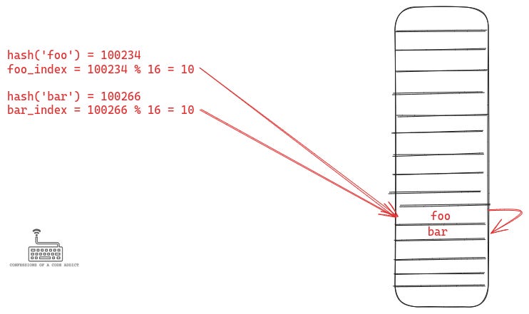
A hash table uses an array as the table for storing and querying the data. But the elements in an array can only be accessed using their index, so hash tables employ a function called the hash function to map the data value to an index in the array, and they store the data item at that index. The following figure illustrates how this works:
The hash function here scans the bytes of the object and maps it to an integer value within a fixed range. An ideal hash function needs to be:
Fast: The hash function should execute quickly so that it does not become a bottleneck in hash table operations.
Uniformly distributed: The hash function should distribute hash values evenly across the entire range, ensuring that each integer value within the range is equally likely to be assigned to a given key. This helps to minimize collisions and ensures efficient use of the hash table.
Minimally correlated: Similar keys should not produce similar hash values. This helps to avoid clustering and ensures that hash table operations remain efficient. In technical terms, the hash function should exhibit a high degree of "avalanche effect," where a small change in the input results in a significantly different output.
We will not discuss the implementation details of the hash function because that is a separate topic in itself. But if you are interested in understanding how such functions are designed, Knuth provides a good exhaustive overview in The Art of Computer Programming, Volume 3, Chapter 6.
However, there is one particular problem that we need to discuss in relation to hash functions, which is that of collisions. Hash collisions happen when two or more objects are mapped to the same hash value.
Unless we are using a perfect hashing scheme, our hash table needs to implement a collision handling measure. Let’s discuss ways to handle collisions next.
Handling Hash Collisions
There are two broad techniques for handling collisions in hash tables:
Chaining: In this method, each position in the hash table points to a linked list (or another data structure) that contains all the items that hash to the same value. When a collision occurs, the new item is simply added to the list at the corresponding position.
Open Addressing: This technique finds an alternate position in the table for storing the colliding item. If a collision occurs, the hash table uses a probing sequence to find the next available slot. Common probing methods include linear probing, quadratic probing, and double hashing.
Separate Chaining
This is one of the most commonly used techniques for handling collisions in hash tables. In this scheme, the entries in the table are converted into pointers to a linked list. When inserting a new data item into the table, the data item is appended to the list at the index generated by the hash function.
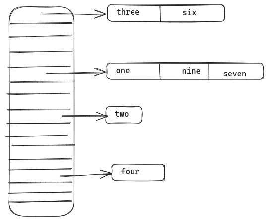
When querying for an item in the table, we have to scan the linked list in the table at the index generated by the hash function. In the ideal scenario, the hash function is good and collisions are rare, so the linked lists will contain very few number of items and can be scanned quickly.
As the number of items in the table grows, the collisions will increase and the linked lists will get longer, thus increasing the time to query the hash table.
Open Addressing Using Linear Probing
Linear probing is one of the simplest and common ways of implementing open addressing. In this scheme, if the current index is occupied in the table, we linearly scan the next consecutive entries in the table until we find an empty slot. If we reach the end of the table, we roll over to the beginning of the table.
Again, there are many more ways of implementing open addressing, such as quadratic probing, double hashing, random probing, but we will not talk about them here.
Separate Chaining vs Linear Probing
In the case of Python’s set implementation, it uses linear probing for its hash table (or rather a combination of linear probing and random probing). They’ve made this choice based on careful performance considerations. Let’s compare the performance characteristics of the two techniques.
Memory Overhead
Separate chaining requires extra memory for storing the objects. For every insertion, we have to allocate a new linked list node, which will start to add up as the table gets larger.
In the case of linear probing (or open addressing in general), there is no such extra memory overhead because it simply uses the array for storing all the objects.
Performance of the Insertion API
Separate chaining can offer fast object insertion into the table, even in the presence of a large number of collisions. Insertion simply requires appending a new node to a linked list, and that is a cheap operation for linked lists.
In the case of linear probing, the insertion can get very slow as the table gets fuller, because we may have to probe a large number of indices in the table until we find an empty slot. A well implemented regrowing strategy can mitigate this.
Performance of Lookups
In the case of separate chaining, lookups can get slower as the table grows. This happens because the linked lists grow longer and longer, and the lookup performance degrades from constant time to linear time (linear in the size of the linked lists).
Similar problem exists with linear probing as well. As the table grows fuller, we would have to probe a large number of entries. However, linear probing is much more cache efficient because we are scanning contiguous indices of the array.
Even if we are trying to load 1 byte of data from main memory, the CPU cache likes to fetch data from the main memory in chunks of 32 or 64 bytes (called the cache line size). So, when doing linear probes we scan one of the array indices, the CPU cache will fetch next several entries into the cache as well. As a result of this, the next few indices of the table will be in the cache and can be compared pretty fast.
Linked lists are not cache friendly, because their nodes are not contiguously allocated in memory.
So overall, from lookups point of view linear probing is usually a much better choice because of better cache locality. Now, let’s dive into Python’s implementation of set.
Definition of Set in CPython
We will start by looking at the definition of the set object in CPython and understanding its memory layout.
The set object is defined in the file setobject.h, and is shown below:
Let’s go over the fields one by one:
Object header: The first field (defined by the macro PyObject_HEAD) is the object header which stores the reference count and type related information. I’ve discussed in this video.
fill: The next field is fill which counts overall how many fillend entries are there in the hash table. This includes the number of active entries and the number of deleted entries from the table. When implementing linear probing, we cannot simply delete an entry, instead we have to mark it as a tombstone (they call it a dummy entry). This is required so that when doing lookups when we encounter a dummy entry in the table, we can continue to probe the next entry, otherwise lookups will start to fail.
used: This counts only the active entries in the table
mask: This is used to map the hash value into the range of the table size. In the hash table section we saw the use of the modulo operator (hash % table_size) for doing this. However, the modulo operator requires division instruction on the CPU which is one of the slower CPU instructions. A more efficient way is to do a bitwise
ANDoperation with a mask. If the table size is a power of 2, then this mask is simply one minus the size of the table, because that value will be all ones (e.g. 7 = 111). Therefore, instead of storing the size of the table, they store this mask value because they need the mask much more frequently than the size itself.table: Table is a pointer to the array which acts the table.
hash: This stores the hash of the set object itself. This is only used when creating a frozenset object, but not used for a regular set.
finger: This field is only used for implementing the
pop()API. Thepop()API deletes an arbitrary element from the set and the value of the finger field dictates which is the element to be deleted.smalltable: This is a static array of 8 entry objects which acts as the table for the set initially. At the time of instantiation, the table pointer points to this small table. This prevents unnecessary allocation of a large array upfront when we don’t even know how many element we will store in the set. As the set size grows, it switches to a dynamically allocated array.
The following illustration shows a more visual memory layout of the set object:
Next, let’s see how a new set object is initialized.
Set Initialization
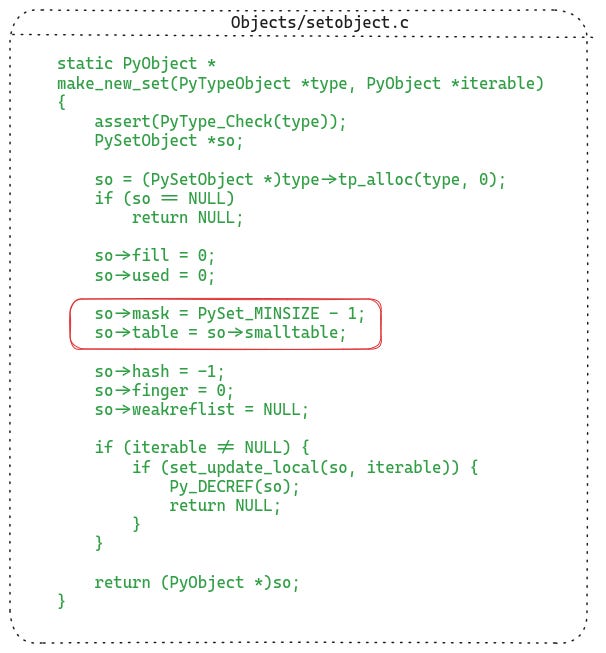
The following listing shows the function which allocates and initializes a new set object:
Most of the details are trivial, but let’s spend a bit of time on the highlighted part.
Initially the set uses the smalltable field as the table (which is an inline allocated array of size 8 in the setobject itself). As the set grows larger, the set object switches to a larger dynamically allocated array.
The mask field is one minus the size of the table. The size of the table is always a power of 2, so that the mask can be used to reduce the hash value within the range of the table size.
For instance, if the table size is 8, then the mask is 7 or 111 in binary. When we have a hash value such as 123, we can reduce it into the table size range by doing 123 & 7 (1111011 & 111 in binary), which gives 3 (011 in binary). This is much faster than using the % operator.
Implementation of Some Critical Set APIs
Now, we can start looking at the implementation of some of the important APIs that the set data structure provides. We will start from insertion or addition of a new object into a set.
Set Insertion API
Computing the Hash of the Object
The first thing which needs to happen is computing the hash of the object that we are trying to add to the set. The following listing shows that part:
That crazy looking if condition is simply an optimization.
Strings in Python are unicode objects and they are immutable. Because of being immutable, Python likes to keep their hash value cached once computed.
So, in the if condition they are checking if this object is a unicode object and if it has a cached hash value, in that case they use that cached hash value and avoid an unnecessary call to the hash function.
However, If the object was not a unicode type, or if it did not have a cached hash value, then they are calling the object’ hash function to compute the hash. Every hashable object in Python needs to implement a hash function, which is what is being called here.
Once, they have the hash value, then they call the set_add_entry function which will do the actual insertion of the object into the set. Let’s take a look at it.
Inserting the Object
We will take a look at the code for inserting the object soon. But first let’s discuss the probing strategy implemented by Python’s set implementation.
We discussed linear probing previously and also talked about how it is CPU cache friendly, which can give better lookup performance in the presence of collisions. The hash table implementation in Python’s set uses a combination of linear probing and random probing.
Initially they do a fix number of linear probes. However, if even after that they are unable to find an available slot in the table, they will use random probing.
In random probing, they simply shuffle the index value using a random function. This function uses the top 5 bits of the hash value, and some additional computation to change the index value. Then the algorithm switches back to linear probing starting at the new index value.
This shuffling of the index to a random value makes sure that there is no clustering of keys to a specific area of the table, and the data is well distributed.
Now, we can look at the actual code for inserting an object into the set. I’ve annotated all the parts, so nothing more for me to write about it.
Set Removal API
Next, let’s take a look at the implementation of the removal API which removes a given object from the set. It is very similar to how objects are added to the set. The first thing they have to do is compute the hash of the object. The following listing shows that code:
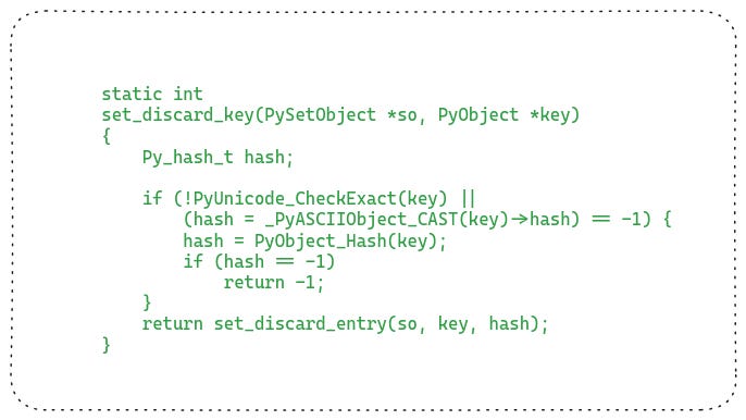
Next, they have to find the entry in the hash table using this hash and remove it. Let’s see its code:
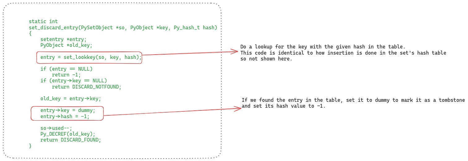
They first do a lookup in the hash table, the algorithm for the lookup is identical to how insertion is done into the set’s hash table that we saw in the previous section.
If they find the key object in the table, then they set that entry in the hash table as a tombstone by setting the hash value to -1.
Set Contains API
Now, the most critical API of the set data structure: the contains API which is used for querying the membership of an object in the set.
At this point, I don’t have to explain anything, I will just show the code:
They compute the hash and then probe the hash table to find the object in it. If they find a match, they return true.
The Set pop API
Finally, I want to show the pop API’s implementation because I think it’s interesting. Python’s set has a pop API which simply removes one arbitrary element from the set. Which element will be deleted is not documented but we can take a look at the code to figure out how the API decides which element to pop.
If you remember, the set object contains a field called finger. The value of the finger field dictates which entry will be deleted from the set. The pop API simply looks up the entry in the hash table pointed to by the finger value and removes it if it is not empty. If that entry is empty, then the algorithm checks the subsequent entries in the table until it finds a used slot and removes it.
At the end, the finger value is set to point to the next slot in the table, i.e. after the entry which just got deleted.
The following listing shows the code:
Thread-Safety of Set APIs
Finally, let’s discuss if Python’s set is thread-safe or not. Until recently, because of the GIL thread-safety was not really a concern because at any point only one thread could be accessing a set object.
However, in the NOGIL build multiple threads can run concurrently. As a result, the set implementation has been made thread-safe. But, it is not really concurrent. All the set APIs, lock the whole object before executing any code. This means that no other thread can perform any operation on that set object while another thread holds the lock.
In a multi-threaded application this can result in a lot of contention and starvation. Hopefully, they will switch to a more concurrent implementation. For instance, Java’s ConcurrentHashMap is a good example which uses more fine grained locking to lock different regions of the table instead of locking the complete table, thus offering improved concurrency.
Overall Impressions of Python’s Set Implementation
There are a lot more APIs that Python’s set supports, such as union, intersection, difference, discard, disjoint. But they are all very similar. In this post we have covered the crucial implementation detail, which is the hash table implementation. I will end this post with some of my final thoughts:
Overall the memory overhead of Python’s set is minimal. It only has the very important and critical fields. The use of an inline array for the initial table is interesting. It saves an extra allocation upfront in the case applications don’t need a large table.
The use of linear + random probing for collision handling is very smart. It gives better lookup performance because of better CPU cache utilization and also prevents clustering of objects.
The current set implementation is not concurrent because it locks the entire object. However, if the GIL is removed from the default build then hopefully they will switch to a more concurrent hash table implementation.
Support Confessions of a Code Addict
If you find my work interesting and valuable, you can support me by opting for a paid subscription (it’s $6 monthly/$60 annual). As a bonus you get access to monthly live sessions, and all the past recordings.
Many people report failed payments, or don’t want a recurring subscription. For that I also have a buymeacoffee page. Where you can buy me coffees or become a member. I will upgrade you to a paid subscription for the equivalent duration here.
I also have a GitHub Sponsor page. You will get a sponsorship badge, and also a complementary paid subscription here.


