A Linear Algebra Trick for Computing Fibonacci Numbers Fast

Fast Fibonacci Computations With a Linear Algebra Twist

Nov 05, 2023

I’ve been attending an online reading group on the book “Thirty-three Miniatures: Mathematical and Algorithmic Applications of Linear Algebra” lead by Prof. Neeldhara Misra from IIT Gandhinagar. It is the most unconventional math book I’ve come across. The first two chapters are all about ways to quickly compute Fibonacci numbers. The conventional (memoization based, or iterative) method of computing Fibonacci numbers that we learn in our programming courses is linear in time. But, the book shows a technique for computing them in approximately logarithmic time complexity. It’s possible that some of you might be aware of this technique but this was news to me and I thought it’s worth sharing with the rest of you.

green leafed plant — Photo by Erol Ahmed on Unsplash

Applying a Linear Algebra Strategy to Fibonacci Number Calculations

The conventional memoized recursive algorithm for computing Fibonacci numbers is this:

table = {}
def fib(n):
    if n in table:
        return table[n]
    
    if n == 0 or n == 1:
        result = n
    else:
        result = fib(n - 1) + fib(n - 2)
    
    table[n] = result
    return result

This is a linear time algorithm because to compute the nth Fibonacci number, we need to compute all the previous n - 1 numbers in the sequence. This leads us to the typical question asked — can we do better?

Let’s try to find out. One issue with the above algorithm is that computing an arbitrary value in the sequence requires us to compute all the previous values. Therefore, we need to arrive at a solution which is more general in nature and can compute the nth value directly.

One intuition we have is that we know the values of the base cases (0 and 1), so if we can express the computation of the nth Fibonacci number in terms of the base cases, we might achieve our goal. Let’s try to build on this intuition.

The base cases of the sequence are:

F(0) = 0
F(1) = 1

Computing F(2) using these two is trivial:

F(2) = F(1) + F(0)

Similarly, we can also express F(1) in terms of F(1) and F(0):

F(1) = 1 * F(1) + 0 * F(0)

We can conveniently express the computation of F(2) and F(1) in a single linear algebra operation, like so:

\(\begin{align} \begin{bmatrix} F(2) \\ F(1) \end{bmatrix} = \begin{bmatrix} 1 & 1 \\ 1 & 0 \end{bmatrix} \begin{bmatrix} F(1) \\ F(0) \end{bmatrix} \\ \\ Or, \begin{bmatrix} F(2) \\ F(1) \end{bmatrix} = \begin{bmatrix} 1 & 1 \\ 1 & 0 \end{bmatrix} \begin{bmatrix} 1 \\ 0 \end{bmatrix} \end{align}\)

Let’s try to do the same thing for F(3):

F(3) = F(2) + F(1)
F(2) = F(1) + F(0)

And representing it in terms of matrix operation, we get this:

\(\begin{bmatrix} F(3) \\ F(2) \end{bmatrix} = \begin{bmatrix} 1 & 1 \\ 1 & 0 \end{bmatrix} \begin{bmatrix} F(2) \\ F(1) \end{bmatrix} \)

However, we know the value of the vector [F(2), F(1)] from the previous step, substituting that value gives us the following:

\(\begin{bmatrix} F(3) \\ F(2) \end{bmatrix} = \begin{bmatrix} 1 & 1 \\ 1 & 0 \end{bmatrix} \begin{bmatrix} 1 & 1 \\ 1 & 0 \end{bmatrix} \begin{bmatrix} 1 \\ 0 \end{bmatrix} \)

Let’s make it simpler:

\(Let's\ represent\ the\ matrix\ \begin{bmatrix} 1 & 1 \\ 1 & 0 \end{bmatrix} as M \)

Which gives us:

\(\begin{bmatrix} F(3) \\ F(2) \end{bmatrix} = M^2 \begin{bmatrix} 1 \\ 0 \end{bmatrix} \)

Looks like we are building a pattern for computing the numbers in terms of the matrix M and the base cases F(1), and F(0). Let’s see if this pattern holds for F(4).

F(4) = F(3) + F(2)
F(3) = F(2) + F(1)

Again, representing these in the form of matrix operations:

\(\begin{align} \begin{bmatrix} F(4) \\ F(3) \end{bmatrix} &= \begin{bmatrix} 1 & 1 \\ 1 & 0 \end{bmatrix} \begin{bmatrix} F(3) \\ F(2) \end{bmatrix} \\ \\ Or, \begin{bmatrix} F(4) \\ F(3) \end{bmatrix} &= M \begin{bmatrix} F(3) \\ F(2) \end{bmatrix} \end{align} \)

Substituting the value of the vector [F(3), F(2)] from the previous computation, we get the following result:

\(\begin{bmatrix} F(4) \\ F(3) \end{bmatrix} = M . M^2 \begin{bmatrix} 1 \\ 0 \end{bmatrix} \)

Which becomes:

\(\begin{bmatrix} F(4) \\ F(3) \end{bmatrix} = M^3 \begin{bmatrix} 1 \\ 0 \end{bmatrix} \)

In general we can find that this pattern repeats and generalizes to this form:

\(\begin{bmatrix} F(n+1) \\ F(n) \end{bmatrix} = M^n \begin{bmatrix} 1 \\ 0 \end{bmatrix} \)

You can also prove to yourself that this holds true using mathematical induction.

Looks like we have an algorithm for computing the nth Fibonacci number without needing to compute all the previous n-1 values in the sequence. However, it requires computing nth power of the matrix M. The naive algorithm for computing powers is also linear in n, which means this algorithm for computing Fibonacci numbers is also linear and we are back to the same spot. But it turns out there are faster ways for computing power, let’s take a look at them.

Computing Powers Quickly

The naive algorithm for evaluating the nth power requires n multiplications and is therefore linear in time. But there are faster algorithms for doing this. For instance, if n is a power of 2 then we can compute M^n by repeated squaring of M, and do it in log2(n) time.

In volume 2 of The Art of Computer Programming, Knuth shows a more generic algorithm for computing x^n. This algorithm relies on the fact that any number can be broken down into sums of powers of 2. For instance, 5 can be written as 2^2 + 2^0, and 9 can be written as 2^3 + 2^0. Therefore, we can write x^n as following:

\(x^n = x^{k_1} * x^{k_2} * x^{k_3}...x^{k_m} \)

Where k1, k2, …, km are powers of 2 which all add up to n.

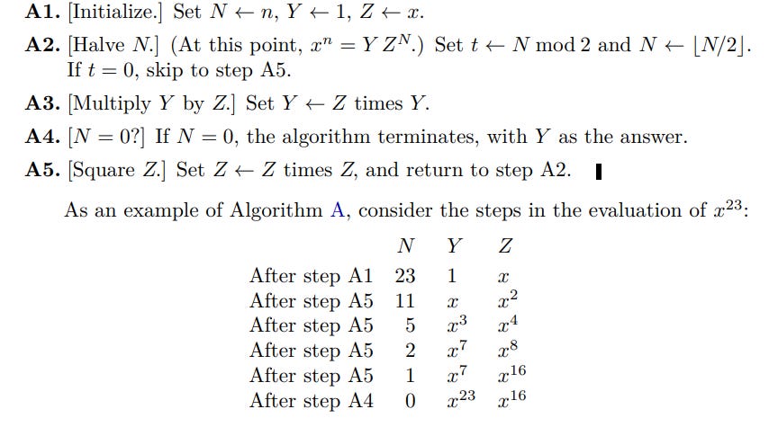
Even though the idea is simple, the actual algorithm for doing this is slightly more convoluted because there is no direct way to break down a number like this. Instead, we need to repeatedly divide the number by 2 and look at the remainder of the result. The 3rd edition of The Art of Computer Programming, Volume 2 (page 462) lists the following algorithm for computing x^n:

Algorithm: For computing x^n. Taken from page 462 of The Art of Computer Programming, Volume 2, Third Edition. — Algorithm: For computing x^n. Based on the algorithm shown on page 462 of The Art of Computer Programming, Volume 2, Third Edition.

If you are someone who prefers looking at code instead of abstract pseudo code, the linalg.matrix_power method in numpy implements this exact same algorithm (shown in the below image).

Numpy implementation of linalg.matrix_power function

What is the complexity of this algorithm? The loop runs no more than log2(n) number of steps because we are halving n at every step. And, during each step of the loop we are multiplying Z by itself, resulting in log2(n) multiplications. Also, whenever we get the remainder as 1, we are also multiplying Z with Y, increasing the number of multiplications. Formally, the total number of multiplications performed by this algorithm is:

\(\lfloor \log_2(n) \rfloor + v(n) \)

Where v(n) is the number of bits with value 1 in the binary representation of n.

This is also the complexity of our Fibonacci number algorithm because the only operation it is doing which depends on n is computing M^n.

It appears we have a more efficient algorithm on our hands. We should actually run and compare the performances of the algorithms before concluding victory. Before we do that, there is another alternative way of computing Fibonacci numbers, let’s look at that.

A Closed Form Expression for Fibonacci Numbers

There is a closed form formula for directly computing the nth Fibonacci number, which uses the golden ratio:

\(F(n) = \frac{1}{\sqrt{5}} \left(\left(\frac{1 + \sqrt{5}}{2}\right)^n - \left(\frac{1 - \sqrt{5}}{2}\right)^n\right) \)

This is probably a much more well known formula, and also derived in The Art of Computer Programming, Volume 1 (page 79). The thirty three miniatures book shows an alternate proof of this form using linear algebra. I would not want to reproduce those proofs here in the interest of space and time, however, feel free to check out those books. I just wanted to show this technique so that we have a more complete benchmark to run. Let’s look at it in the next section.

Comparing Different Fibonacci Number Algorithms

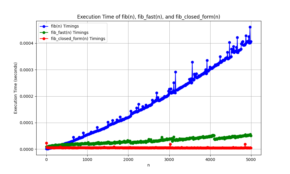
So we have three different algorithms for computing Fibonacci numbers, it’s time we put them to test and compared their performances. The following plot shows the performance of the three techniques.

Execution time of the three algorithms for computing Fibonacci numbers for increasing values of n

Here:

fib(n) refers to the conventional linear time algorithm.
fib_fast(n) refers to the faster algorithm we studied in 2nd section, which computes M^n.
fib_closed_form(n) shows the performance of the closed form formula based on the golden ratio.

This is a great example of the performance difference of linear vs logarithmic time algorithms. Compared to the performance of the linear time algorithm, the other algorithms look like flat lines.

Another interesting thing to note here is the performance of fib_fast and fib_closed_form algorithms. Both of these algorithms essentially compute the nth power of an expression and therefore their complexities in terms of n are same. However, the golden ratio based algorithm is computing the nth power of a scalar value which can be done much faster than computing the nth power of a 2X2 matrix, thus the difference in their actual run-time performance.

At the same time, it is also worth noting that the closed form formula is working with irrational numbers which can only be represented approximately in computers, and thus in some rare cases the method may produce incorrect result due to approximation errors. The matrix method has no such issues and will always give the right answer. Of course, when implementing any of these algorithms you need to handle the possibility of large numbers, which may cause overflow on fixed-width data types.

Wrapping Up

This brings us to the end of this whirlwind tour of Fibonacci number algorithms. When I first came across the linear algebraic formula for computing Fibonacci numbers, I found it magical. The author of the thirty three miniatures book, Matoušek, mentions that the original source of that technique is not known, so we may never know how was it discovered. I believe that when playing around with such sequences, you discover certain patterns which may lead you down the path of such discoveries, and there might not be an exact science behind how it was arrived at. I tried to show one way of how it could be arrived at but there might be better ways to do it. If any of you have better intuition behind it, please share with me in the comments.

Expressing Gratitude

I would like to credit Prof. Neeldhara Misra for leading the session on this topic and for providing intuition behind the math involved. If you are interested on discussions around CS and Math, you may want to follow her on X/Twitter.

I would also like to thank

Alejandro Piad Morffis

for reviewing and giving feedback on this article. He writes a wonderful Substack on topics related to computer science at

Mostly Harmless Ideas

, you may want to check it out and subscribe!